Inferring unknown unknowns: real-time bias-aware data assimilation
There is a variety of statistical methods in data assimilation, which can be broadly classified into variational (e.g. 4DVar), or sequential methods (e.g. Kalman filters). The choice of method depends on the specific application and the characteristics of the system being studied. Sequential methods are also referred to as real-time data assimilation because the observations are processed on-the-fly as soon as they become available. This is an iterative procedure in which observations are continually collected, and the model states and/or parameters are repeatedly adjusted to incorporate the new data. In a nutshell, the assimilation process consists of repeating sequentially the following three steps:
- Forecast: propagate the numerical model in time until observation data become available. The model provides an estimate of the observed physical quantity, which is known as the forecast.
- Analysis: combine optimally the forecast with the observations. This results in an improved estimate of the physical quantity, which is more accurate than the forecast, and it is known as the analysis.
- Update: the analysis state becomes the initial condition for the next forecast step.

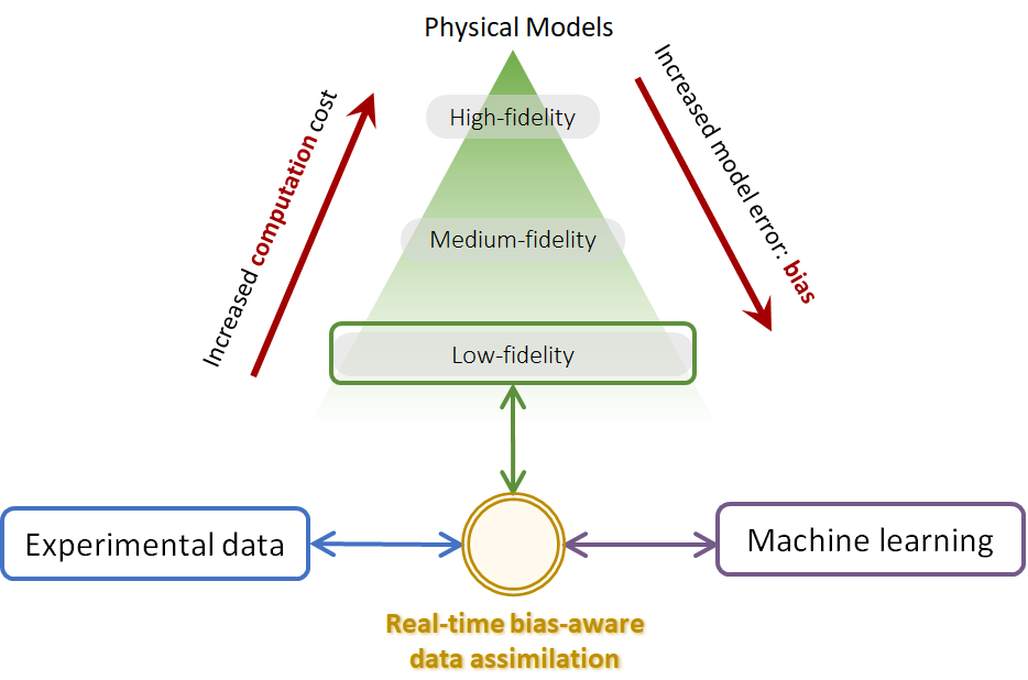
In order to apply real-time data assimilation to low-fidelity models, we must provide an estimate of the bias in the numerical model, i.e., the model error that we introduce when simplifying the physical equations. But, how do we estimate the evolution of the bias? The model error is an unknown unknown, which may be a function of the physical state, the surroundings or even a function of time.
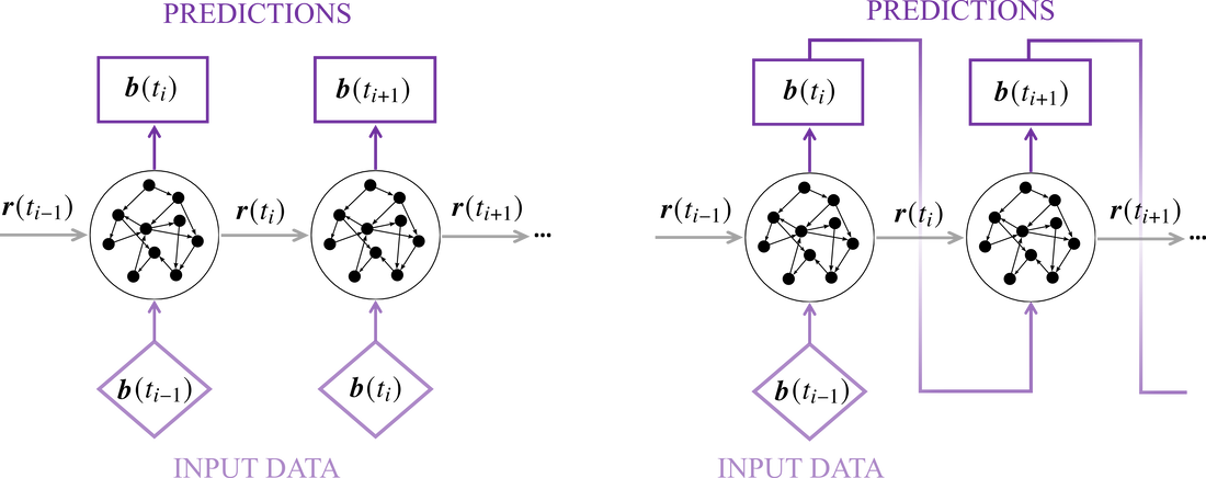
Recent advances in machine learning for data-driven modelling allow us to develop surrogate models of dynamical systems using neural networks. This is, we can use a neural network to estimate the bias of the low-order numerical models. Particularly, we have proposed Echo State Networks (ESNs) for this real-time task because their training consists of a computationally-cheap linear regression problem (see Chaotic time series forecasting). The architecture of the model bias estimation by ESN is illustrated below. The network can evolve in open-loop (left) when observations are available; or in closed-loop (right), in which the ESN runs autonomously.
- Forecast: propagate the imperfect numerical model in time to provide a biased forecast when observation data become available.
- Bias-correction: provide an estimate the bias, and project the biased forecast into an unbiased forecast.
- Assimilation: combine optimally the unbiased forecast with the observations. The direct assimilation results in an unbiased analysis, and the biased analysis is an indirect by-product of the assimilation.
- Update: the biased analysis is the initial condition for the new forecast step.
We aim to estimate a physical quantity in nature with a low-order numerical model \(\mathbf{F}\), which is a function of model parameters and state vafriables represented by \(\boldsymbol{\psi}\); and an operator \(\mathbf{M}\), which maps \(\boldsymbol{\psi}\) into the obsercable state, such that \begin{align}\nonumber \dfrac{\mathrm{d}\boldsymbol{\psi}}{\mathrm{d} t} &= \mathbf{F}\left(\boldsymbol{\psi} \right), \\ \label{eq:problem} \boldsymbol{y} &= \mathbf{M}\boldsymbol{\psi} + \boldsymbol{b} + \boldsymbol{\epsilon} \end{align} where \(\boldsymbol{y}\) is the unbiased model estimate, i.e., the model estimate corrected with the estimate of the model bias \(\boldsymbol{b}\). The aleatoric uncertainties in the model parameters and states, as well as the uncertainties in the operator \(\mathbf{M}\) are combined into the stochastic noise \(\boldsymbol{\epsilon}\), which is assumed to be Gaussian in time.
We use real-time data assimilation to improve our knowledge in the system's parameters and states. With biased models, assimilation methods may be ill-posed because either (i) they are ‘bias-unaware’ because the estimators are assumed unbiased, (ii) they rely on an a priori parametric model for the bias, or (iii) they can infer model biases that are not unique for the same model and data. Real-time methods for nonlinear complex physical models are commonly formulated in a Kalman filter framework using an ensemble approach. Within the ensemble approach, the state and parameter estimation are is achieved by forecasting a number of \(m\) simulations, such that the model \(\mathbf{F}(\boldsymbol{\psi}_j)\) propagates each ensemble member to forecast states \(\boldsymbol{\psi}_j^\text{f}\). Mathematically, we pose the problem by regularizing the traditional data assimilation cost function such that
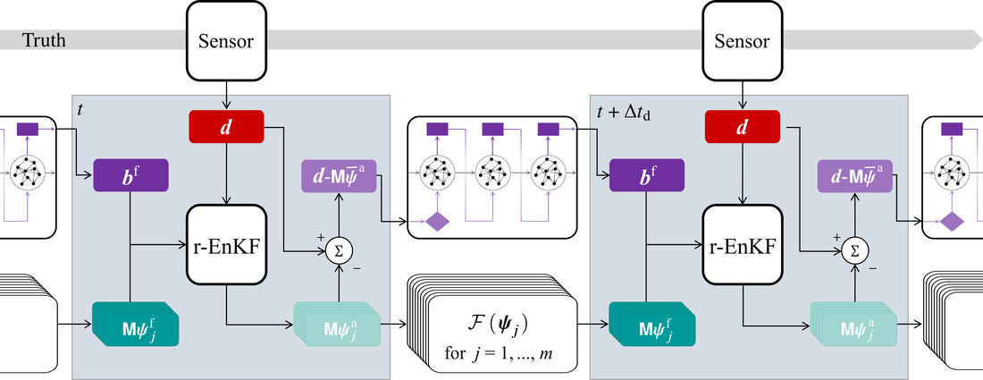
When a sensor provides noisy data \(\boldsymbol{d}\), we apply the r-EnKF, which statistically combines the noisy data, the ensemble mean bias, and the forecast ensemble. The r-EnKF results in the analysis ensemble of states, \(\boldsymbol{\psi}_j^\text{a}\), which are new initial conditions for \(\mathcal{F}\); and the analysis innovation \(\boldsymbol{d}-\mathbf{M}\overline{\boldsymbol{\psi}}^\text{a}\) re-initialize the ESN. This process is repeated sequentially every \(\Delta t_\text{d}\) time between observations.
- Research funded partially by EPSRC, Cambridge Trust, and Rolls-Royce.
- Nóvoa, A., Racca, A. & Magri, L. (2023). Inferring unknown unknowns: Regularized bias-aware ensemble Kalman filter. Computer Methods in Applied Mechanics and Engineering, 418, 116502.
- Nóvoa, A., & Magri, L. (2022). Real-time thermoacoustic data assimilation. Journal of Fluid Mechanics, 948, A35.
- The code used for this project is publicly available on GitHub.


