Nonlinear reduced order modelling
What is reduced order modelling?
In many scientific fields, such as fluid mechanics and atmospheric modeling, physical phenomena are complex and computationally expensive to model. To decrease the complexity of the problem, reduced order modelling (ROM) is typically sought. Reduced order models are simpler, yet accurate, approximations of the system, which provide insights on the physics and predict the evolution of the system at a lower computational cost.
What is nonlinear reduced order modelling, a bit more technically?
Fluid dynamics systems are computationally expensive to simulate because of they are modelled by the Navier-Stokes equations, which can have up to 10^10 degrees of freedom. To deals with such immense systems, reduced-order models aim to find a lower-dimensional representation of the problem, onto which the dynamics can be accurately simulated at lower computational cost.
In particular, nonlinear reduced order models are obtained when using nonlinear projections to lower the dimensionality of the system. In doing so, they differ from traditional methods, such as proper orthogonal decompisition (POD) and principal component analysis (PCA), which reduce the dimensionality of the data through matrix multiplication, i.e., a linear projection.
Among the different ways to nonlinearly lower the dimensionality of the system, machine learning, in the form autoencoders, provides a flexible methodology that has been extensively shown to outperform POD/PCA. In the autoencoder architecture, different layers, e.g., feed-forward, convolutional or graph, are applied to the data in an unsupervised way to compress (encoder) the input to a lower-dimensional representation, the latent space, and then to decompress (decoder) the latent representation back to the physical space, trying to recover the input.
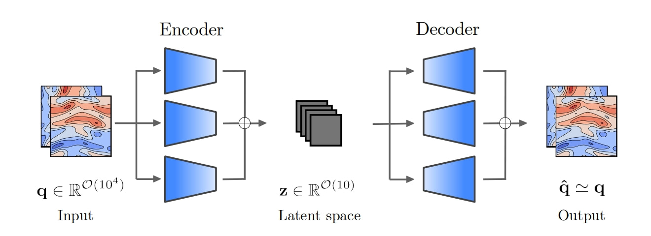
Schematic representation of an autoencoder. The flow is compressed to a lower-dimensional representation, the latent space, thorugh the encoder, and then decompressed back to the physical space through the decoder.
Once the latent space is generated, we wish to predict the temporal dynamics within the latent space. This is a non-trivial task, as the equations in the latent space differ from the equations in physical space. To model the evolution of the system in the latent space, we use recurrent neural networks, which are networks specfically designed to predict time series and sequential data. Because the networks predict orders of magnitude fewer degrees of freedom with respect to the original system, solving the ROM is significantly faster than simulating the original system.
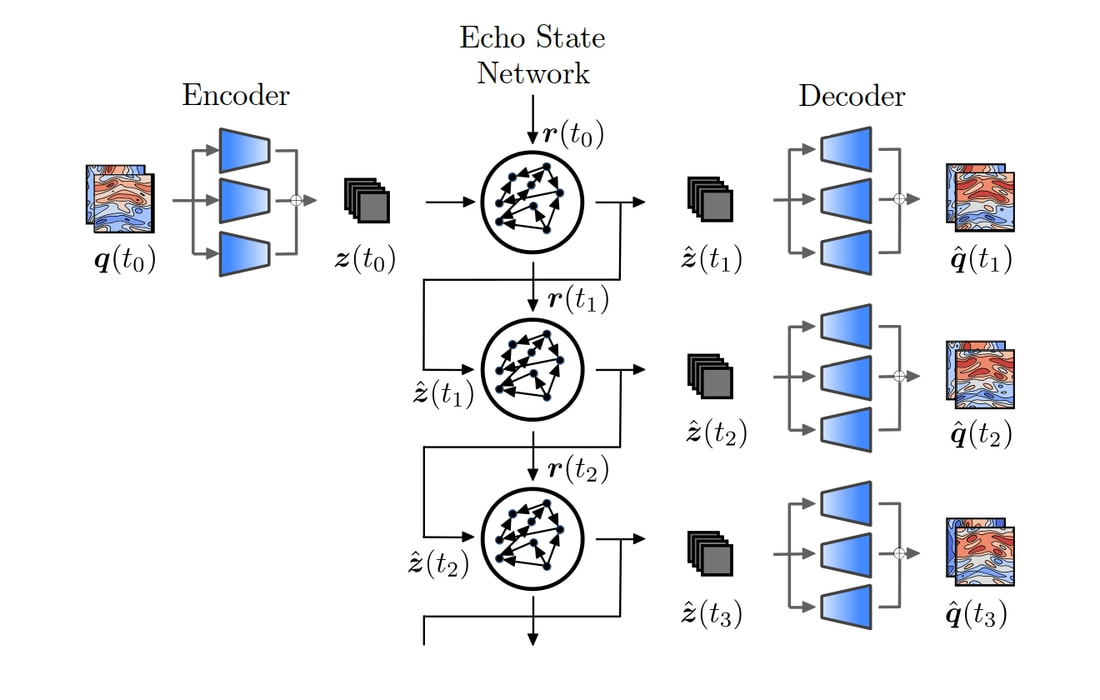
Example of nonlinear ROM, the CA-ESN. The echo state network, a type of RNN, predicts the evolution the latent space dynamics, which are then decompressed by the decoder.
An example of practical application: Predicting turbulence from data
We construct a nonlinear reduced order model to predict the dynamics of the 2D Kolmogorov flow in quasiperiodic and turbulent regimes.
Because the testcase shows spatio-temporal dynamics, we build the autoencoder using convolutional layers, which are designed to handle spatially varying data, such as images and flowfields. Through the autoencoder, we generate the mapping from (and back to) the flowfield to a low-rder representation. The convolutional autoencoder (CAE) is able to find an accurate mapping for small latent spaces, here measured through the reconstructed energy of the flowfield (Energy = 1 means exact reconstruction). The CAE markedly outperforms POD in all cases analysed, providing a more accurate reconstruction with 9 latent space variables than POD with 100 latent space varibales.
Because the testcase shows spatio-temporal dynamics, we build the autoencoder using convolutional layers, which are designed to handle spatially varying data, such as images and flowfields. Through the autoencoder, we generate the mapping from (and back to) the flowfield to a low-rder representation. The convolutional autoencoder (CAE) is able to find an accurate mapping for small latent spaces, here measured through the reconstructed energy of the flowfield (Energy = 1 means exact reconstruction). The CAE markedly outperforms POD in all cases analysed, providing a more accurate reconstruction with 9 latent space variables than POD with 100 latent space varibales.
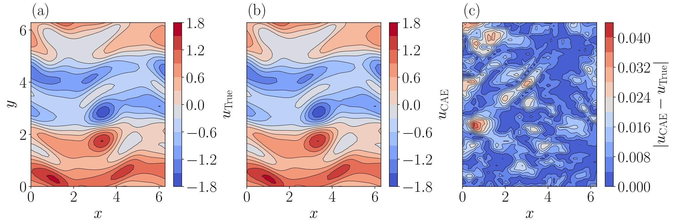
Reconstruction of the velocity along x in a snapshot of the turbulent Kolmogorov flow. The CAE (b) accurately recovers the input (a).
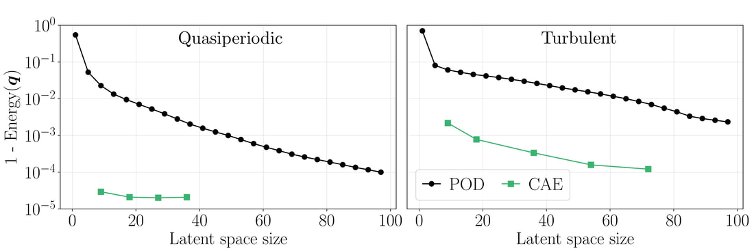
Accuracy of the reconstruction with the convolutional autoencoder (CAE). The CAE markedly outperforms POD in both quasiperiodic and turbulent regimes.
Now that the CAE provides the mapping to the latent space, we want to predict the time evolution in the lower dimensional space. We do so by merging an echo state network with the autoencoder, into the CAE-ESN, which accurately predicts the future evolution of the system for large times.
Finally, because the CAE-ESN evolves in time by predicting only a small fraction (O(10^{-2}-10^{-3})) of the original degrees of freedom, it is more than two order of magnitude faster than the original solver.
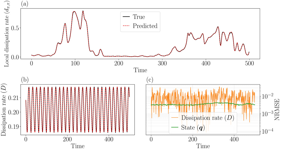
Prediction of the CAE-ESN in the quasiperiodic case. Starting from an initial point at t0, the CAE-ESN evolves autonomously, i.e., without requiring any data, up to 500 time units. In the entire interval, the prediciton of (a) the local and (b) the global dissipation rates is accurate, as further shown through the error in (c).
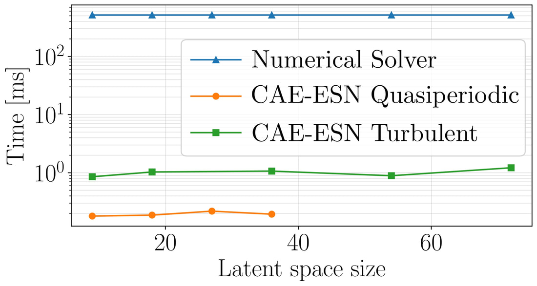
Computational time required to solve the Kolmogorov flow for 1 time unit. The CAE-ESN is more than two orders of magnitude faster than the numerical solver in alla cases analysed. A single GPU is used for all cases.
Material, activities, and people
This work was part of the PhD of Alberto Racca. It is published in
Predicting turbulent dynamics with the convolutional autoencoder echo state network, A.Racca et al., JFM (2023).
The implementation of the CAE-ESN, including a tutorial of the architecture, is publicly available on GitHub.
Research funded by EPSRC, Cambridge Trust and ERC grants.
An example of practical application:
Nonlinear decomposition of wind tunnel experiments
Nonlinear decomposition of wind tunnel experiments
AEs compress data nonlinearly into the latent space, providing a higher compression ratio than linear methods like POD. However, the results are also less interpretable. Our project aims to link POD to the latent space so we can build nonlinear ROMS while guided by flow physics.
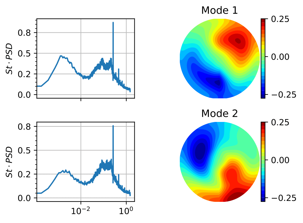
We first analyse the latent space of a compressed laminar unsteady wake. The flow is periodic in time and could theoretically be represented by a single variable. The frequency content of the flow contains a fundamental frequency and its harmonics (multiples of the fundamental frequencies.
By training multiple AEs with different latent dimensions, we find that at least two latent variables are needed to represent periodic data. When there are too few latent variables, unphysical frequencies from numerical tricks show up in the latent space; when there are too many latent variables, multiple latent variables will share physical interpretations unnecessarily.
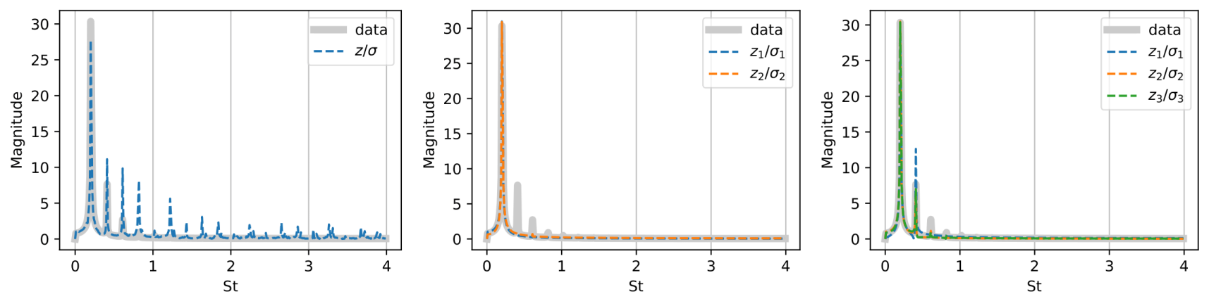
The frequency content of the latent variables z from AEs of different latent dimensions compared to the frequency content of the laminar unsteady flow, normalised by their standard deviation. Left: AE with a single latent variable, contains unphysical frequencies. Middle: AE with two latent variables, contain only the fundamental frequencies. Right: AE with three latent variables, some latent variables contain both the fundamental frequency and the first harmonic to the fundamental frequency.
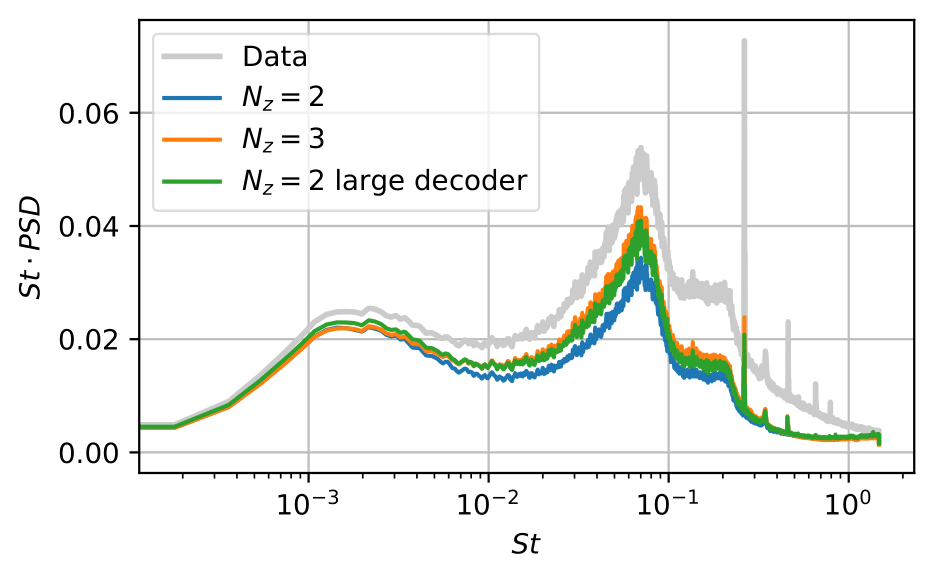
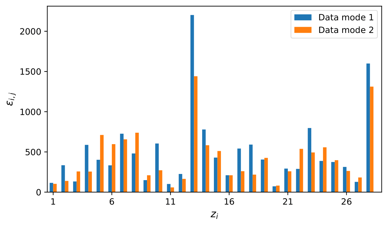
We then analyse the latent space of a compressed turbulent experimental wake of an axisymmetric body. The details of the dataset can be found in the papers by (Rigas, Morgans and Morrison, 2015; Rowan D. Brackston, 2017).
In addition to the importance of the latent dimension we find with the laminar dataset, we learn that the size of the AEs is also a bottleneck for turbulent data with complex spatial structures. Starting with a smaller AE, we find that doubling the size of the decoder has the same effect as having an additional latent variable. The takeaway message is that the latent dimension may not be the ideal physical low-dimensional representation of the data because the AE may not be big enough, leading to the effects of numerical tricks being included in the latent space to improve approximation.
Since POD modes are commonly regarded as coherent structures, we can use POD modes to rank and select latent variables for our ROMs.
We first project the AE's prediction onto the POD modes to relate the latent space to the coefficients of POD modes. We then compute the average rate of change in the POD mode due to the latent variables by taking derivatives. The average rate of change tells us how important is each latent variable for modelling the POD modes, aka the coherent structures. By using only the two most important latent variables for the POD modes representing vortex shedding, we can control the prediction of the AE so that only vortex shedding is modelled.
References:
Rigas, G., Morgans, A.S. and Morrison, J.F. (2015) ‘Stability and coherent structures in the wake of axisymmetric bluff bodies’, in. Cham: Springer International Publishing (Instability and control of massively separated flows), pp. 143–148. Available at: http://link.springer.com/10.1007/978-3-319-06260-0_21.
Rowan D. Brackston (2017) Feedback Control of Three-Dimensional Bluff Body Wakes for Efficient Drag Reduction. Imperial College London. Available at: https://doi.org/10.25560/52406.
Material, activities, and people
This work is part of the PhD of Yaxin Mo, in collaboration with Tullio Traverso.
All codes and implementation can be found on GitHub, at https://github.com/MagriLab/MD-CNN-AE.
This work is part of the PhD of Yaxin Mo, in collaboration with Tullio Traverso.
All codes and implementation can be found on GitHub, at https://github.com/MagriLab/MD-CNN-AE.